Please read the previous post: The ‘Gentle’ introduction to hartree fock first. After reading that post you should be aware that basis functions are a crucial aspect of the method and the challenge is evaluating the various integrals involved. This post seeks to give a clearer picture on the details of the gaussian basis orbitals and the recusive integration schemes involved.

My colab notebook, basis orbital(STO3G) csv and some xyz files of simple molecules can be found at:https://drive.google.com/drive/folders/1pgo2eG_R51U1eiHy3NXE7Bj8OS_NgNL0?usp=sharing. Feel free to check it out. The code has implemented the schemes which I have described below.

1. A recap on the integrals

Based on the previous introduction, there are 4 main integrals of interest:

1. Overlap integral, \(S_{\mu v} = \int \psi_{\mu}\psi_v dr\)
2. Kinetic Integral, \(T_{\mu v} = -\frac{1}{2} \int\psi_{\mu}\nabla^2\psi_v dr\)
3. Nuclear attraction integral, \(V_{\mu v} = – \sum_{inuc = 1}^{Nnuc}\int\psi_{\mu}\frac{Z_{inuc}}{|r – r_{inuc}|}\psi_v dr\)
4. The exchange/coulomb tensor: \((\mu v| \lambda \sigma) = \int\int \psi_{\mu}(r_1)\psi_v(r_1) \frac{1}{|r_1-r_2|}\psi_{\lambda}(r_2)\psi_{\sigma}(r_2)dr_1 dr_2\)

They have been listed in increasing order of difficulty and the last integral is the most tedious to calculate. I have derived these integrals myself and I will give a separate and very lengthy post on the derivation. But before I mention the integrals, I should first explain the gaussian basis set.

2. The gaussian basis and virtual orbitals

The basis orbitals used in molecular Hartree Fock are Atomic Orbitals. Every atom in the molecule, carries a certain number of basis orbitals. For the simplest basis set: STO-3G and STO-2G, Hydrogen carries 1x 1s basis orbital, Nitrogen carries 1 x1s, 1x 2s and 3x 2p orbitals and so on. You get the idea. For every atom, the AOs used are basically \(\approx\) the Atomics orbitals on the gaseous atom. For more advanced basis sets, the number of basis orbitals per atoms is significantly more as there are polarisation orbitals – additional basis orbitals per atom which alows for more variation to the shape of the molecular orbtials – and hence gives a larger basis set. I understand that I have not touched on a crucial point in my prev post. That is the number of basis orbitals used are probably > number of filled shells/number of spin orbitals(UHF). Well then during the diagonalisation, the number of eigenvectors and eigenvalues(the number of molecular orbitals and energies) the process spits out = number of basis orbitals involved. The density operator only takes into account the orbitals that are filled and hence when the method calculates the exchange interactions, they are correct. However, what are the empty orbitals and their energies? Well, it is mostly an artifact of the program as a result of using more basis orbitals than there are filled ones. But they do give a semi decent estimation of the energy gaps between the gnd state and the first excited state and their orbitals have close symmetry to the occupied excited molecular orbitals. Infact, using TDHF and TDDFT, these vacant orbitals are used along with the filled orbitals to approximate the excited states, but I will cover these on a much later date. The reason why gaussian orbitals are gaussian is that they are approximated by a linear sum of gaussians. For STO-3G, every orbital is approximated by a sum of 3 gaussians and some of the more complicated basis sets will have around 5 to 6 gaussian orbitals and 3 or more polarising functions per basis function. Having gaussian functions greatly simplify the calculations as explained below

3. The properties of Gaussian orbitals

An orbital centered on atom at R has tjhe following form:

\(\psi_R(r) = (x-R_x)^a(y-R_y)^b(z-R_z)^c \sum_{i=1}^{3}c_i N_i e^{-\alpha_i (r-R)^2}\)

And \(c_i\) is the contraction coefficientsn while \(N_i\) are the nomalization constants for each gaussian involved. Typically, the polynomial part of the orbital is applied to all gaussians and hence, the for mula for the normalisation constant is:

\(N = (\frac{2\alpha}{\pi})^{3/4}\frac{(4\alpha)^(a+b+c)/2}{\sqrt{(2a-1)!!\times (2b-1)!!\times (2c-1)!!}}\)

where !! denotes the double factorial. Whenever 2 gaussians are multiplied tgt, the result is still a gaussian. Consider \(e^{-\alpha (r-A)^2}\times e^{-\beta (r-B)^2}\). The resulting gaussian is:

\(K_{\alpha,\beta} \times e^{-p(r-P)^2}\)

where \(P = \frac{\alpha A +\beta B}{\alpha + \beta}\) and \(p = \alpha +\beta\) and \(K_{\alpha,\beta} = exp(-\frac{\alpha \beta}{\alpha + \beta}|A-B|^2)\). With this in mind, I can now layout the integral schemes.

4. The Overlap and Kinetic Integrals

Both these use the same scheme with the exception that Kinetic is alittle more complex and has a few more terms to calculate for each matrix element. For the STO-3G, each orbital has 3 gaussian functions and hence there are a total of 9 sub integrals to sum over for the overlap integral. The general sturcture of each integral(btw any 2 gaussians) is:

\(c_A c_B N_A N_B \times \int product of polynomial terms \times gaussian product\)

The 2 gaussians used here to demonstrate the general case for atoms A and B are:

\((x-A_x)^{a_1}(y-A_y)^{a_2}(z-A_z)^{a_3}exp(-\alpha|r-A|^2)\)

\((x-B_x)^{b_1}(y-B_y)^{b_2}(z-B_z)^{c_3}exp(-\beta|r-B|^2)\)

The contraction terms and normalisation constants need to be included infront! The terms within the integral will look something like this:

\((x-A_x)^{a_1}(y-A_y)^{a_2}(z-A_z)^{a_3} (x-B_x)^{b_1}(y-B_y)^{b_2}(z-B_z)^{c_3}\times K_{\alpha,\beta} \times e^{-p(r-P)^2}\)

But the integral can be separated into the different coordinates since \(exp(-p|r-P|^2)\) can be separated into: \(exp(-p|x-P_x|^2)\times exp(-p|y-P_y|^2\times exp(-p|z-P_z|^2))\). This trick recurs across all integrals later and the only integrals that need to be considered are one dimensional integrals of the form:

\(\int (r_i-A_i)^{a_i}(r_i-B_i)^{b_i}exp(-p(r_i-P_i)^2)\)

Denoting such 1D integrals as \((a_i,b_i)\) then the general formula for the integral btw any 2 gaussians is:

\(c_A c_B N_A N_B K_{\alpha,\beta}\times (a_x,b_x)\times (a_y,b_y)\times (a_z,b_z)\)

Now the general scheme to evaluate the 1D integrals given the necessary exponents and positions of the gaussian centers, the 2 recursion relations are as follows:

VRR: \((a_i+2,0) = (P_i-A_i)(a_i+1,0) + \frac{a_i+1}{2p}(a_i,0)\)

HRR: \((a_i,b_i+1) = (a_i+1,b_i) + (A_i-B_i)(a_i,b_i)\)

In this case, I have set \(p = \alpha +\beta\) and \(P = R’\)(defined earlier). The starting 2 terms in this recursion are:

\((0,0) = \sqrt{\frac{\pi}{p}}\) and

\((1,0) = (P_i – A_i)\sqrt{\frac{\pi}{p}}\)

And the general scheme to get to any combination of \((a_i,b_i)\) is given by:

1. First use the VRR and the first 2 terms to generate all the terms from \((a_i,0)\) to \((a_i+b_i,0)\)
2. Use the HRRs to generate terms from \((a_i,1)\) to \((a_i+b_i-1,1)\)
3. sucessive HRRs on this list will generate \((a_i, k)\) to \((a_i+b_i-k,k)\) until the list is down to just(a_i, b_i)

Summarised in the following diagram for the example (a,3):

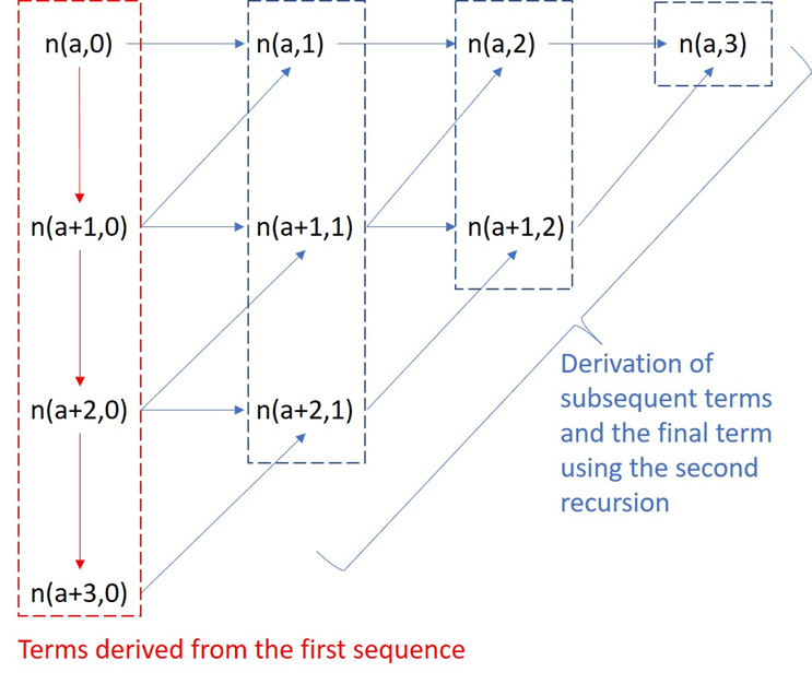
Note that since \(\sqrt{\frac{\pi}{p}}\) is a common factor in all integrals so it could be factored out first before doing the recursion and the first 2 terms would be 1 and \(P_i – A_i\). For the case of STO 3G where a basis orbital has the form:

\(\psi_{v} = (x-A_x)^{a_1}(y-A_y)^{a_2}(z-A_z)^{a_3}\sum_{g}^3c_gN_g e^{-\alpha_g |r-A|^2}\)

Then a term in the overlap matrix will look something like(when I have factored out \(\sqrt{\frac{\pi}{p}}\) from the integrals):

\(S_{\mu v} = \sum_{g1}\sum_{g2}c_{g1}c_{g2}N_{g1}N_{g2}K_{g1,g2}(\frac{\pi}{p})^{3/2} (a_x,b_x)(a_y,b_y)(a_z,b_z)\)

For the case of the kinetic integral, there are also 9 main integrals but their structure is different. Due to the \(\nabla^2 =\partial_x^2 +\partial_y^2+\partial_z^2\) each of the 9 integrals are broken up into 3 terms, one for each 1d laplacian. hence, given the same example gaussian orbitals introduced earlier, the following integrals need to be calculated 9 times:

\(I_x = (\frac{\pi}{p})^{3/2}(4\beta^2(a_x+2,b_x)-2\beta(2b_x+1)(a_x,b_x)+b_x(b_x-1)(a_x,b_x-2))(a_y,b_y)(a_z,b_z)\)

\(I_y = (\frac{\pi}{p})^{3/2}(4\beta^2(a_y+2,b_y)-2\beta(2b_y+1)(a_y,b_y)+b_y(b_y-1)(a_y,b_y-2))(a_x,b_x)(a_z,b_z)\)

\(I_z = (\frac{\pi}{p})^{3/2}(4\beta^2(a_z+2,b_z)-2\beta(2b_z+1)(a_z,b_z)+b_z(b_z-1)(a_z,b_z-2))(a_x,b_x)(a_y,b_y)\)

And hence, the final kinetic energy element is given by:

\(T_{\mu v} = -\frac{1}{2}\sum_{g1}\sum_{g2}c_{g1}c_{g2}N_{g1}N_{g2}K_{g1,g2}(I_x+I_y+I_z)_{g1,g2}\)

5. Nuclear Repulsion Integral

Now with the first 2 integrals out of the way, I can get to the nuclear integral. For one nucleus and 2 basis orbitals, it is essentially just a modified overlap integral and this has to be repeated for every nucleus. So for every nucleus and 2 basis orbitals, there will be 9 terms to calculate for STO-3G and the total number of terms for one \(V_{\mu v}\) is 9x number of Nuclei, and the number will be higher for more advanced basis sets. The derivation is more tricky and I unfortunately wont go over it but I will leave it in a later post. For ease of understanding, lets use the same 2 example gaussians:

\((x-A_x)^{a_1}(y-A_y)^{a_2}(z-A_z)^{a_3}exp(-\alpha|r-A|^2)\)

\((x-B_x)^{b_1}(y-B_y)^{b_2}(z-B_z)^{c_3}exp(-\beta|r-B|^2)\)

And lets just calculate the integral of the product multiplied by the nuclear coulomb term for a nucleus at R: \(-\frac{Z_{nuc}}{|r-R|}\). The result needs to be calculated numerically and it is:

\(\frac{2\pi}{p}K_{\alpha,\beta}\int_{0}^{1}e^{-t^2p|P-R|^2}n_x(a_x,b_x,t)n_y(a_y,b_y,t)n_z(a_z,b_z,t)dt\)

And the integrals \(n_i(a_i,b_i,t)\) are derived through the following recursion relations:

VRR: \(n_i(a_i+2,0,t) = ((P_i-A_i)-t^2(P_i-R_i))n_i(a_i+1,0,t) + \frac{a_i+1}{2p}n_i(a_i,0,t)\)

HRR: \(n_i(a_i,b_i+1,t) = n_i(a_i+1,b_i,t) + (A_i-B_i)n_i(a_i,b_i,t)\)

The first 2 terms are: \(n_i(0,0,t) = 1\) and \(n_i(1,0,t) = (P_i-A_i)-t^2(P_i-R_i)\). These recursion relations are basically the same as the earlier schemes with the annoying issue that polynomial multiplication is involved. The slow computation method is the symbolic way, the fast way is the polynomial multiplication through vector convolution which is intuitive. And the final step is the numerical evaluation of an exponetial integral which is actually quite simple to evaluate if the correct approximations are used. I will return to this later once I cover the next section on the 4 orbital tensor evaluation which also requires similar steps. Notice that this is the result for just the integral between 2 gaussians and the nuclear term. Hence, denoting this integral btw the gaussians(g1,g2) and the \(i_{nuc}^{th}\)nuclei as \(I_{g1,g2,inuc}\), the full expression for an arbitrary \(V_{\mu v}\) is given by:

\(V_{\mu v} = \sum_{inuc}\sum_{g1}\sum_{g1}c_{g1}c_{g2}N_{g1}N_{g2}K_{g1,g2}I_{g1,g2,inuc}\)

With this out of the way, it is time to move on to the final and most challenging integral – the electron repulsion tensor.

6. Electron exchange integrals/tensor

Finally, I have arrived at the most difficult integral to evaluate – the electron exchange integral. This is more difficult due to the 1/r term having both \(r_1,r_2\) followed by a double integration over both coordinates makes this a 6 dimensional integral.

A key difference from the other terms is that the integral requires only 2 basis orbitals per element since 2d tensor but this is 4d so plenty.

Anyway, the same tricks used in the previous integral are used and I will be using the 4 gaussians below as an example of how one such integral looks like:

\((x-A_x)^{a_1}(y-A_y)^{a_2}(z-A_z)^{a_3}exp(-\alpha|r-A|^2)\)

\((x-B_x)^{b_1}(y-B_y)^{b_2}(z-B_z)^{c_3}exp(-\beta|r-B|^2)\)

\((x-C_x)^{a_1}(y-C_y)^{c_2}(z-C_z)^{c_3}exp(-\gamma|r-C|^2)\)

\((x-D_x)^{d_1}(y-D_y)^{d_2}(z-D_z)^{d_3}exp(-\delta|r-D|^2)\)

The new gaussian produced from gaussians A and B is given by: \(K_{\alpha \beta}exp(-p|A_B|^2)\) and the gaussian produced from gaussians C and D is given by: \(K_{\gamma \delta}exp(-q|C-D|^2)\) where \(p = \alpha +\beta \) and \(q = \gamma + \delta\). The new centers of the 2 gaussians are \(P\) and \(Q\) respectively. The expression for the double integral is:

\(I_{ABCD} = \frac{2\pi^{5/2}}{pq\sqrt{p+q}}\int_{0}^{1}e^{t^2\rho|P-Q|^2}(a_x,b_x,c_x,d_x)(a_y,b_y,c_y,d_y)(a_z,b_z,c_z,d_z)dt\)

Where \(\rho = \frac{pq}{p+q}\) and the recursive relations for the integrals, \((a_i,b_i,c_i,d_i)\) are:

1. the 2 VRRs:

\((a_i+1,0,c_i,0) = A_{00}(a_i,0,c_i,0)+a_iA_{1}(a_i-1,0,c,0)+c_iB_{00}(a_i,0,c_i-1,0)\)

\((a_i,0,c_i+1,0) = C_{00}(a_i,0,c_i,0)+a_iB_{00}(a_i-1,0,c,0)+c_iC_{1}(a_i,0,c_i-1,0)\)

With the polynomial coefficients defined as:

\(A_{00} = (P_i – A_i) -\frac{qt^2}{p+q}(P_i-Q_i), C_{00} = (Q_i – C_i) +\frac{pt^2}{p+q}(P_i-Q_i)\)

\(A_{1} = \frac{1}{2p}(1-\frac{qt^2}{p+q}), C_{1} = \frac{1}{2q}(1-\frac{pt^2}{p+q})\)

\(B_{00} = \frac{t^2}{2(p+q)}\)

2. The 2 HRRs:

\((a_i,b_i+1,c_i,d_i) = (a_i+1,b_i,c_i,d_i)+(A_i-B_i)(a_i,b_i,c_i,d_i)\)

\((a_i,b_i,c_i,d_i+1) = (a_i,b_i,c_i+1,d_i)+(C_i-D_i)(a_i,b_i,c_i,d_i)\)

Evidently, navigating to any term is a challenge but first, a quick note on the evaluation of a single term \((\mu v|\lambda \sigma)\). This involves 4 orbitals and hence, if every orbital comprise 3 gaussians then the evaluation of just one term will require 3^4 of these 4 gaussian integrals. I have calculated these integrals recursively in python tho it may not be very efficient and I have some schemes implemented in a colab code which I will post the link to later. Do let me know if you have any suggestions on a faster algorithm for evaluating this tricky tensor. But with that I have finally come to the end of this article.

Some After thoughts

Well learning Hartree Fock wasnt exactly very straightforward for me especially since I began this more than 2 years ago before I even had any formal University education. I had to get by with bits and pieces of information from various textbooks or online resources. For a more indepth discussion on the method and introduction to some computational chemistry do look up modern quantum chemistry by szabo and ostlund which is a good resource and it includes an example with H2 if I recall correctly. The main purpose of doing this blog post is to give you guys some help when evaluating the integrals exactly. I remember I couldnt really find clear concise summaries of the various recursions required for the different integrals and I had to work through the entire derivations by myself to arrive at the results I have presented earlier. You can also check out joshuagoing’s notes which I didnt have access to a few years back but those also present similar integration schemes. In my implementation online, they seem to give pretty similar results to pyscf and I think my calculations are correct. Pls let me know if there are any corrections and I hope you had a great time learning about the actual implementation of the procedure.