Cyclostationary Signal processing is a rather niche area of Signal processing and it is mainly used in determining the cyclostationary statistics of a signal. What exactly are cyclostationary properties, you may ask. Think of it simply as a statistical property of the signal(like perhaps the mean or even the variance) which happen to vary periodically with time. For example, the expected value of the temperature for the day 15 Nov 2025 may not be similar to that for the day 1 October 2025. However, it will probably be very similar to that for the day 15 Nov 2025. This is just one example to help visualise what an example of such a cyclostationary statistic could be. When it comes to digital signal processing, some modulation types, especially the digital modulations may modulate the signal periodically, giving rise to strong cyclostationary properties. Some good examples are:

1. Amplitude modulation: the amplitude of the signal vaaries periodicially with time
2. BPSK modulation: a bit rate of 500bits/sec will flip the phase by 180 degrees at that rate

As for cricket songs, which I am very used to analysing, the chirp rate will create modulations in both amplitude and carrier frequency(although small ~ 10 to 100Hz). Now you may ask then how exactly is this analysed?

The Cyclic Autocorrelation Function

The Autocorrelation function most readers are familiar with is the ordinary autocorrelation function:

\(R_{x}(t,\tau) = E[x(t+\tau/2)x^*(t-\tau/2)]\)

Usually the expectation can be sampled from the value of the signal directly and it is given by:

\(R_{x}(t,\tau) = \lim_{T\to\infty}\frac{1}{T}\int_{-T/2}^{T/2} x(t+\tau/2)x^*(t-\tau/2)dt \)

Notice that I have included the variable \(t\) here to denote the central time around which the autocorrelation is done and \(\tau\) is the lag between the two signals. For signals with no cyclostationary statistics(an ordinary sine wave for example), the value of this autocorrelation would NOT depend on the parameter \(t\). However, for cyclostationary statistics, \(R_{x}(t,\tau)\) would vary periodically with t. Hence, in the autocorrelation can be written as a fourier series:

\(R_{x}(t,\tau) = \sum_{\alpha} R_{x}^{\alpha}(\tau)e^{2\pi i \alpha t}\)

The fourier coefficients of the autocorrelation \(R_{x}(\tau)\) is given by the cyclic autocorrelation function(CAF)(\(R_{x}^{\alpha}(\tau)\)):

\(R_{x}^{\alpha}(\tau) = \lim_{T\to\infty}\frac{1}{T}\int_{-T/2}^{T/2} R_{x}(t,\tau)e^{-2\pi i \alpha t} dt\)

Due to cycloergodicity, the necessary coefficients can be extracted directly from the time series using:

\(R_{x}^{\alpha}(\tau) = \lim_{T\to\infty}\frac{1}{T}\int_{-T/2}^{T/2} x(t+\tau/2)x^*(t-\tau/2)e^{-2\pi i \alpha t} dt\)

And there you have it, the cyclic autocorrelation function, its simple interpretation and a numerical way to estimate it. In practice, with digital signal processing, the signal is usually recorded over time in discrete bins and hence the shifts in time need to be discrete as well.

\(R_{x}^{\alpha}[l] = e^{\pi i \alpha l} \langle x[m]e^{-2\pi i\alpha m} x^*[m-l] \rangle\)

Here, the bins \(m,l\) run from \(0\) to \(N-1\) where N is the length of the signal segment recorded. If there is only one realisation(like one sample of length N) of the signal being used to estimate the CAF(this is not recommended as the noise will be bad), then \(\alpha = [-N//2,…,N//2]/N\). Usually the CAF will be averaged through the use of sliding windows:

1. The entire signal of duration \(N\) is broken up into sliding windows of length \(N_p\) and a shift between windows(\(L\)) of \(N_p/4\)
2. For each window, the CAF is calculated as above with \(m,l \in [0,N_p – 1]\) BUT the \(\alpha\) values are still given by the expression: \(\alpha \in [-N//2,…,N//2]/N\)
3. The last step before averaging is the phase correction for each window for each value of $\alpha$

It may seem unintuitive that the resolution for the cyclic frequency is still determined by the length of the whole window \(N\) and why phase correction needs to be done. A simple way to understand the first result is that for cyclic frequencies, they are essentially ‘measured’ and deduced from the more long term trend of the entire signal series. Hence, the resolution is determined by the total signal length of the entire window. As for the phase correction, the CAF of the \(p^{th}\) window will be phase shifted with respect to the CAF for the \(0^{th}\) window by a phase shift:

\(e^{2\pi i \alpha pL}\)

Thus, for the \(p^{th}\) window, I have to correct for each \(\alpha\) by multiplying the entire row/column(depending on how you made your CAF tensor) by the correct phase factor: \(e^{-2\pi i \alpha pL}\) This ensures that all estimates of the CAF are at the same phase and averaging the CAF removes any remaining phase noise.

The Spectral Correlation Function(SCF)

Before I show any plots on the result, I will try to cover an alternative method which is related to the CAF. The Spectral Correlation Function(SCF) is the fourier transform of the CAF over the \(\tau\) parameter:

\(R_{x}^{\alpha}(\tau) \leftrightarrow S_{x}^{\alpha}(f)\)

The SCF is also related to the cyclic periodogram of a signal, \(I_{T}(u,f,\alpha)\) which is typically defined as:

\(I_{T}(u,f,\alpha) = \frac{1}{T}[X(f+\alpha/2)X^*(f-\alpha/2)]\)

Here, \(T\) is the duration of the time window used to make this periodogram and the cyclic periodogram is a single estimate of the correlation between frequency components in a signal with central frequency \(f\) and difference of \(\alpha\). To compute the true SCF, one has to calculate many instances of the cyclic periodogram and average them. For example, with a time-smoothing method, the calculation will resemble:

\(S_{x}^{\alpha}(f) = \lim_{T\to\infty}\lim_{U\to\infty}\frac{1}{U}\int_{-U/2}^{U/2}I_{T}(t,f,\alpha)dt\)

This function is plotted as its modulus square and the 2 axis will be \(\alpha,f\). Key features of an \(|S_{x}^{\alpha}(f)|^2\) plot:

1. \(\alpha = 0, S_{x}^{0}(f)\) corresponds to the ordinary frequency power spectrum of the signal.
2. For any 2 correlated frequency components(\(f_1,f_2\)), not only will they have peaks at \(\alpha = 0\), there will be a significant SCF value at \(\alpha = \pm|f_2-f_1|\) and \(f = \frac{f_1+f_2}{2}\).

That roughly sums up the main features to look out for in an SCF plot and I think this should suffice for an introduction on how to interpret the SCF plot.

Some examples and explanations

I have some examples of CAFs and SCFs with real world data. I have some cricket songs and the structure of a cricket song is that it contains a series of chirps, usually repeated at a regular interval. A simple example is shown below:

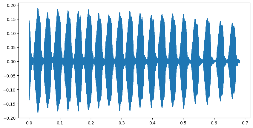
Every pulse you see here is basically one chirp and it is caused by the single opening and closing of the crickets wing – and throughout the entire process, the wings vibrate very quickly giving rise to fast oscillations modulated by a much more slowly varying envelope. When crickets sing, many species repeat the chirp at a relatively fast past giving rise to a trill as shown in the figure. The chirp repetition rate(C.R.R) can then be picked up by the CAF and SCF which usually shows strong amplitudes at \(\alpha = \)C.R.R. For the signal above, the relevant diagrams are shown below:

Thus, the pulse repetition rate of ~ 30Hz shows up quite obviously on the SCF and higher harmonics appear too! The main reason for whether higher harmonics appear has to do with fourier analysis which essentially states that any function periodic with period \(T\) can be represented using a sum of sinusoidal functions with frequencies\(\propto n/T\). The number of harmonics involved depends on the shape of the envelope of the chirp. For a hypothetical rectangular pulse, higher harmonics of the basic pulse repetition rate will show in the diagram and for smoother, more sinusoidal-like pulses, the number of harmonics seen will be fewer. This can be illustrated with the calling song of a mole cricket, Gryllotalpa nymphicus:

Its pulses are smoother and as such the SCF and CAF have fewer cyclic components:

In this song, there is only one really dominant cyclic frequency at ~120Hz followed by a much weaker 2nd harmonic at ~240Hz. But this interestingly implies that the mole cricket songs are approximately modelled by a central carrier sine wave @~2300-2400Hz modulated by a sine wave envelope at frequency (60Hz). I am indeed really excited to share more examples but that would make this post really long. Readers interested in trying some of these techniques can access my signal processing notebook and relevant files at this google drive folder and for a gallery of the results, you can checkout my gallery page.

An alternative route to the SCF, the FFT Accumulation Method(FAM)

The FFT Accumulation method is an alternative to getting the SCF. This method also involved averaging the SCF over multiple windows but it si way more computationally efficient. It achieves this in two different FFTs, the first FFTs is performed over all windows and the second one, over all different frequency pairs(more on this later). The first FFT has a computational complexity ~ \(O(P N_plog(N_p))\) and the second FFT has the complexity of \(O(N_p^2Plog(P))\). In here, \(P\) = total number of windows used, \(N_p\) = length of each window. The following algo is designed such that \(P\), \(Np\) are all powers of 2. A quick summary of the processes of the FAM are:

1. First FFT which gives the Frequency Spectrum for each window.Builds a tensor  with dimensions \((P,N_p)\)

2. Each column in the tensor is multiplied by the conjugate of another column(could be itself too)

3. FFT over this result is the equivalent of averaging(the zeroth component). The Frequency resolution of this 2nd FFT is \(\frac{f_s}{LP}\) where L is the shift between windows. Instead of just adding the zeroth component to the final SCF tensor, a small segment around the zeroth frequency is added to allow for interpolation and smoothing of the SCF Function.

To see more of this algorithm in action, I have included a few cells in my colab notebook with the code adapted from https://pysdr.org/content/cyclostationary.html#fft-accumulation-method-fam. With that, I have come to the end of this introductory post on cyclostationary signal processes and have playing around with my colab notebook. I am very grateful to Chad Spooner for pointing out mistakes in my orignal formulas and I have learnt a great deal from his blog at https://cyclostationary.blog/about/. If you are interested in topics that I have not covered here – such as the conjugate CAF and SCF, or higher-order cyclic cumulants – I highly recommend reading his posts.