Hartree Fock is an ab initio method used to calculate the molecular orbitals and their energies of a given molecule. This is an extremely powerful tool since the chemical and physical properties of the molecule can be inferred before the experiment is performed. In this post I hope to detail the underlying physics regarding the calculation and give and overview of how the method works. I will be focusing mainly on Restriced Hartree Fock(Closed shell molecules) there will be another post detailing the exact implementation including how the various orbital integrals are evaluated explicitly.

My colab notebook, basis orbital(STO3G) csv and some xyz files of simple molecules can be found at: https://drive.google.com/drive/folders/1pgo2eG_R51U1eiHy3NXE7Bj8OS_NgNL0?usp=sharing. Feel free to check it out.

1. The basics:

The Hartree Fock is essentially calculating the wavefunction for the electrons of a given molecule. I would strongly recommend anyone reading this to familiarise themselves with basic quantum mechanics first. Since the electrons are fermions, they obey the pauli exclusion principle. Therefore their total wavefunction is antisymmetric under the exchange of any 2 particles’ labels. Let \(\Psi(r_1,r_2,r_3,…,r_i,…,r_j,…r_N)\) be the wavefunction of N such fermions(in the positional representation). The pauli exclusion principle implies that for any value of i and j:

\(\Psi(r_1,r_2,r_3,…,r_i,…,r_j,…r_N) = – \Psi(r_1,r_2,r_3,…,r_j,…,r_i,…r_N)\)

Thus, this also implies that if 2 particles occupy the same state, the only valid wavefunction that can obey the antisymmetry rule is when the wavefunction vanishes and this results in the pauli exclusion principle. Now the question is given N fermions and N single particle states, how can the overall wavefunction be made to be symmetric? This can be done using what is called a slater determinant. Imagine having the single particle states: \(\chi_i\) and the coordinates of the fermion:\(r_j\). The slater determinant would look something like:

Usually most closed shell molecules have a single slater determinant describing their entire wavefunction. The issue becomes more complicated with Open Shell Molecules since their wavefunctions are typically a linear combination of several slater determinants. Hartree Fock in its original formulation assumes that the molecular wavefunction is a single slater determinant. For pedagological reasons, I will continue with the single slater determinant wavefunction as it is way easier to undertsand and it captures most of the essence of Hartree Fock. Now, since we have the structure of the wavefunction, it is time to consider the hamiltonian. The many particle hamiltonian will have the following form:

\(\langle H\rangle= \sum_{i=1}^{N}\langle \Psi | h_i |\Psi \rangle + \sum_{i=1}^{N}\sum_{i<j}^{N} \langle \Psi | \frac{1}{r_{ij}} |\Psi \rangle\)

Where \(h_i = -\frac{1}{2}\nabla_i^2 -\sum_{k=1}^{N_{nuc}}\frac{Z_k}{r_{ik}}\), the single particle hamiltonians which measure each fermion’s own kinetic energy and the potential energy due to nuclear attraction. The second term is basically the coulomb repulsion term between all unique pairs of fermions. However, to do any calculation with this is very messy and it would be more optimal to reformulate the problem interms of the single particle orbitals involved without ever needing to use the labels of the individual particles.

It can be shown that the single particle hamiltonian terms simplify to give:

\(\sum_{i=1}^{N}\langle \chi_i |h| \chi_i \rangle\)

Where \(h = -\frac{1}{2}\nabla^2 -\sum_{k=1}^{N_{nuc}}\frac{Z_k}{|r-r_k|}\). Thus, the expectation energy of the system ignoring electron-electron repulsion is simply the sum of the single particle orbital energies. The remaining electron electron term is then rearranged as:

\(\sum_{i<j}^{N,N}[ii,jj]-[ij,ij], [ij,kl] = \int dr_1 dr_2 \chi_i^*(r_1)\chi_j(r_1)\frac{1}{r_{12}}\chi_k^*(r_2)\chi_l(r_2)\)

The Hartree Fock method is essentially a variational method and the ground state is found by minimising the expectation energy w.r.t the orbitals. Treating this as a lagrange optimisation problem gives the following equation to solve:

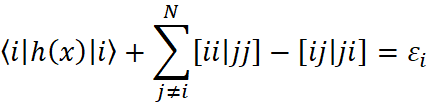
Solving this equation gives $lates \varepsilon_i$, the orbital energies of the ith molecular orbital. This energy can be measured as the ionisation energy of that orbital: energy required to remove an electron from that orbital and bring it to infinity. Now solving this problem is way easier than the original equation but before i cover that, a quick notes on the units used.

I have used atomic units in the derivation and you can work it out to see how they reduce the hamiltonians to the simpler forms used above. In atomic units:

1. energy units: the hartree, \(E_{hartree} = \frac{\hbar^2}{m_e a_0^2}\)
2. distance units: bohr radius, \(a_0\)

There are more units but these 2 fundamental conversions give the hamiltonians above.

2. The approach with basis orbitals

The equations while easier to solve are still not very easy to solve. Finding the exact shape of the molecular orbitals is non-trivial and thus, an approximate workwaround is used for this method. Intead of finding the exact function of the molecular orbitals, why not just approximate each with a linear combination of basis orbitals. Given a certain basis set of orbitals, the ith molecular orbital will have the form:

\(\chi_i = \sum_{v = 1}^{K}C_{vi}\psi_v\)

With this in mind, the operators(hamiltonian) can be written in terms of the basis. Usually the basis orbitals are atomic orbitals(AOs) but in periodic structures, plane waves would be more appropirate. Before the hamiltonian can be written in terms of the basis orbitals, the hamiltonian needs to be re written as an operator. Currently, it is not a single particle operator in its equation form. The \(h\) operator can be easily pulled out but the interaction terms are a challenge. Forutnately, we are standing on the shoulders of giants and they have found a neat way to do so.

The 4 orbital integral defined earlier is:

\([ij,kl] = \int dr_1 dr_2 \chi_i^*(r_1)\chi_j(r_1)\frac{1}{r_{12}}\chi_k^*(r_2)\chi_l(r_2)\)

and the 2 integrals of interest are \([ii,jj], [ij,ji]\). The first operator called the coulomb operator is defined as such:

\(J_j(x_1) = \int dx_2 \frac{1}{r_{12}}\chi_j^{*}(x_2)\chi_j(x_2)\)

Thus, taking the expectation of this operator with any molecular orbital(\(\chi_i(x_1)\)) gives \([ii,jj]\). The next operator, the exchange operator can be defined similarly:

\(K_j(x_1) = \int dx_2 \frac{1}{r_{12}}\chi_j^{*}(x_2) P_{12} \chi_j(x_2)\)

In this form, \(P_{12}\) is the exchange operator which exchanges the dummy coordinates of the 2 functions behind it. Thus, taking the expectation value of \(K_j\) with any molecular orbital(\(\chi_i(x_1)\)) returns \([ij,ji]\). With this in mind, the ‘single particle’ hamiltonian operator aka the Fock operator is:

\(F = -\frac{1}{2}\nabla^2 -\sum_{k=1}^{N_{nuc}}\frac{Z_k}{|r-r_k|} + \sum_{j}^{N}[J_j-K_j]\)

There is something interesting about this operator in the sense that it is non-linear and thus, finding the eigenvalues and eigenvectors in terms of the basis orbitals is a non-linear eigenvalue problem. The most obvious source of non-linearity are the coulomb and exchange operators which depend on the other eigenvectors. An interesting thing to note is that the original sum \(\sum_{i\neq j}^{N}[ii,jj]-[ij,ij]\) now runs over the whole list of j from 1 to N since when i = j, the $lates J_j$ and \(K_j\) operators cancel. With the fock operator formalised, we are now ready to cast it in terms of the basis orbitals. Consider any molecular orbital \(\chi_i\), then it follows that:

\(F\chi_i = \chi_i \varepsilon_i\)

In terms of basis orbitals, this is:

\(\sum_{v=1}^{K}F\psi_v C_{vi} = \sum_{v=1}^{K}\psi_v C_{vi}\varepsilon_i\)

Next, multiplying by \(\psi^*_{\mu}\) and then integrating over the space gives:

\(\sum_{v=1}^{K}F_{\mu v} C_{vi} = \sum_{v=1}^{K}S_{\mu v} C_{vi}\varepsilon_i\)

This is infact equivalent to the matrix equation: \(FC = SC\varepsilon\) where \(F_{\mu v}\) and \(S_{\mu v}\) are the matrix elements of F and S respectively in the basis orbital basis and \(\varepsilon\) is the diagonal matrix of molecular orbital energies. The elements are written explicitly as:

\(F_{\mu v} = \int \psi^*_\mu F \psi_v dx\)

\(S_{\mu v} = \int \psi^*_\mu \psi_v dx\)

If F did not contain the repulsion terms then solving this would just be solving a generalised eigenvalue problem. The introduction of the S matrix is necessary since not all basis orbitals are orthogonal to each other. The S matrix is clearly hermitian. While the S elements are easily evaluated, the F elements arent trivial. \(F_{\mu v}\) can be separated into 2 parts, a linear part corresponding to the kinetic energy and nuclear potential energy and yes, the dreaded interaction tensor:

\(F_{\mu v} = H_{\mu v} + \sum_{j}^{N}\int \psi^*_{\mu}[J_j – K_j]\psi_v dx\)

\(H_{\mu v} = T_{\mu v} + V_{\mu v} \)

\(T_{\mu v} = -\frac{1}{2}\int\psi^*_{\mu}\nabla^2\psi_v dx \)

\(V_{\mu v} = -\sum_{i_{nuc}}^{N_{nuc}} \int\psi^*_{\mu} \frac {Z_{inuc}} {|r-r_{inuc}|}\psi_v dx \)

The coulomb operator can be rewritten in terms of basis orbitals first:

\(J_j = \int \sum_{\lambda}^{K} C^*_{\lambda j}\psi^*_{\lambda}(x_2) \sum_{\sigma}^{K} C_{\sigma j}\psi_{\sigma}(x_2) \frac{1}{r_{12}}dx_2 \)

now letting \(C^*_{\lambda j} C_{\sigma j} = P^j_{\lambda \sigma}\) then the sum of \(J_j\) gives:

\(\sum_{\lambda,\sigma}^{K,K} P_{\lambda \sigma}\int\psi^*_{\lambda}(x_2)\psi_{\sigma}(x_2) \frac{1}{r_{12}}dx_2 \)

Where \(P_{\lambda \sigma} = \sum_{j}^{N}P^j_{\lambda \sigma}\). Finally, the next integration with \(\psi^*_{\mu} and \psi_v\) to get the matrix element is:

\((\sum J_j)_{\mu v} = \sum_{\lambda,\sigma}^{K,K} P_{\lambda \sigma} (\mu v|\lambda \sigma)\)

Applying thr same logic to \(K_j\) and taking into account the effect of the swapping operator gives:

\((\sum K_j)_{\mu v} = \sum_{\lambda,\sigma}^{K,K} P_{\lambda \sigma} (\mu \sigma|\lambda v)\)

Now all operators have been successfully expressed interms of the basis orbitals and solving can begin. It is clear that F depends on C and thus the general steps are:

1. First find all relevant tensors like S, T, V.
2. Using an initial guess of C, find F and solve the generalised eigenvalue equation
3. Using the returned eigenvector matrix, C build the density operator P again and compare it with the previous value
4. If the deviation is still significant, then feed the P back into F and repeat solving the generalized eigenvalue problem
5. The process repeats until the density operator P of prev iterations agree well.

Above is the formulation for the general case. With closed shell molecules, the formulation is slightly easier but I should clarify some of the integrals used above. In all inegrals listed above, they are integrations over a product space: position space x spin. The orbitals involved are spin orbitals. Hence, when summing over K, it sums over all basis orbitals and when the sum over j is performed for the coulomb and exchange operators, it only goes over the occupied molecular orbitals(single particle orbitals with the lowest energies). The integral \((\mu \sigma|\lambda v)\) has the form:

\(\int dx_1 dx_2 \psi_\mu^*(x_1)\psi_\sigma(x_1)\frac{1}{r_{12}}\psi_\lambda^*(x_2)\psi_v(x_2)\)

Thus, basis orbitals of orthogonal spin will lead to 0 overlaps which removes some terms. This comes in very handy especially in the Restricted Hartree Fock method.

3. Restricted Hartree Fock

With the RHF, pure spatial basis orbitals are typically used. This makes book keeping much easier especially with the vector space spanned by the basis orbitals much smaller. The eigenvectors returned by this method are the spatial representations of the molecular orbitals in the basis. The fock operator changes as follows:

\(F_{\mu v} =H_{\mu v} + \sum_{j=1}^{N/2}[2J_j – K_j]_{\mu v} \)

Where N is the total number of electrons in the system and since the molecule is closed shell, the number of spatial orbitals to be summed over is N/2. The reason for the factor of 2 for the coulomb operator(for spatial orbital basis) is that the electron in a particular orbital can interact with any other electron regardless of spin of the other electron. But the exchange operator is only non-zero if the 2 orbitals in consideration are of the same spin state. Hence, the coulomb interaction has twice the number of interactions as the exchange operator. The negative sign also implies that it is energetically favourable for the molecule to adopt a maximum spin state and align unpaired electrons, consistent with Hund’s rule. But anyway, there is no change to \(H_{\mu v}\) and the coulomb exchange operators for the RHF just become:

\(\sum_{\lambda,\sigma}^{K,K} P_{\lambda \sigma} [(\mu v|\lambda \sigma)-\frac{1}{2}(\mu \sigma|\lambda v)]\)

And the density operator is now calculated as: \(P_{\lambda \sigma} = 2\sum_{j}^{N/2}C^*_{\lambda j}C_{\sigma j}\). Now all integrations prev defined for spin orbitals are now replaced byintegrations over purely spatial orbitals.

4. Finding \(\langle H \rangle\) of the system

Now that most of the formalism for the RHF architecture has been detailed, it is time to review the original problem. While knowing the molecular orbitals and energies are important, what is the energy of the system as a whole? Surely it is not the naive sum of the molecular orbital energies since there are interaction terms and that would be double counting. First, summing over the energy eigenvalues of the filled orbitals is done through:

\(\sum_{\mu v}^{K,K}P_{\mu v}H_{\mu v}\)

And then the Coulomb and exchange energies are given by:

\(E_{coulomb} = \frac{1}{2} [P_{\mu v} P_{\lambda \sigma} \times (\mu v| \lambda \sigma)]_{sum}\)

\(E_{exc} = -\frac{1}{4} [P_{\mu v} P_{\lambda \sigma} \times (\mu \sigma| \lambda v)]_{sum}\)

And the last term to be included is the internuclear repulsion(easily calculated using classical electrostatics):

\(E_{tot} = T_{tot} + V{tot}+E_{coulomb}+E_{exc}+E_{rep,nuc}\)

With that I have come to the end of my ‘Gentle’ Introduction to Hartree Fock with a focus on the RHF method. I will be updating this post from time to time to make it clearer and in an upcoming post, I will detail how the orbital integrations are done with the gaussian orbital basis which gives recursive analytical results making the method fast and efficient. One a note on complexity, constructing the tensor \((\mu v| \lambda \sigma)\) scales as \(O(N^4)\) and this tensor is the main scaling challenge behind this method. In a future I may also cover the formalism for the UHF method which is able to handle molecules with unpaired electrons and so stay tuned for more!